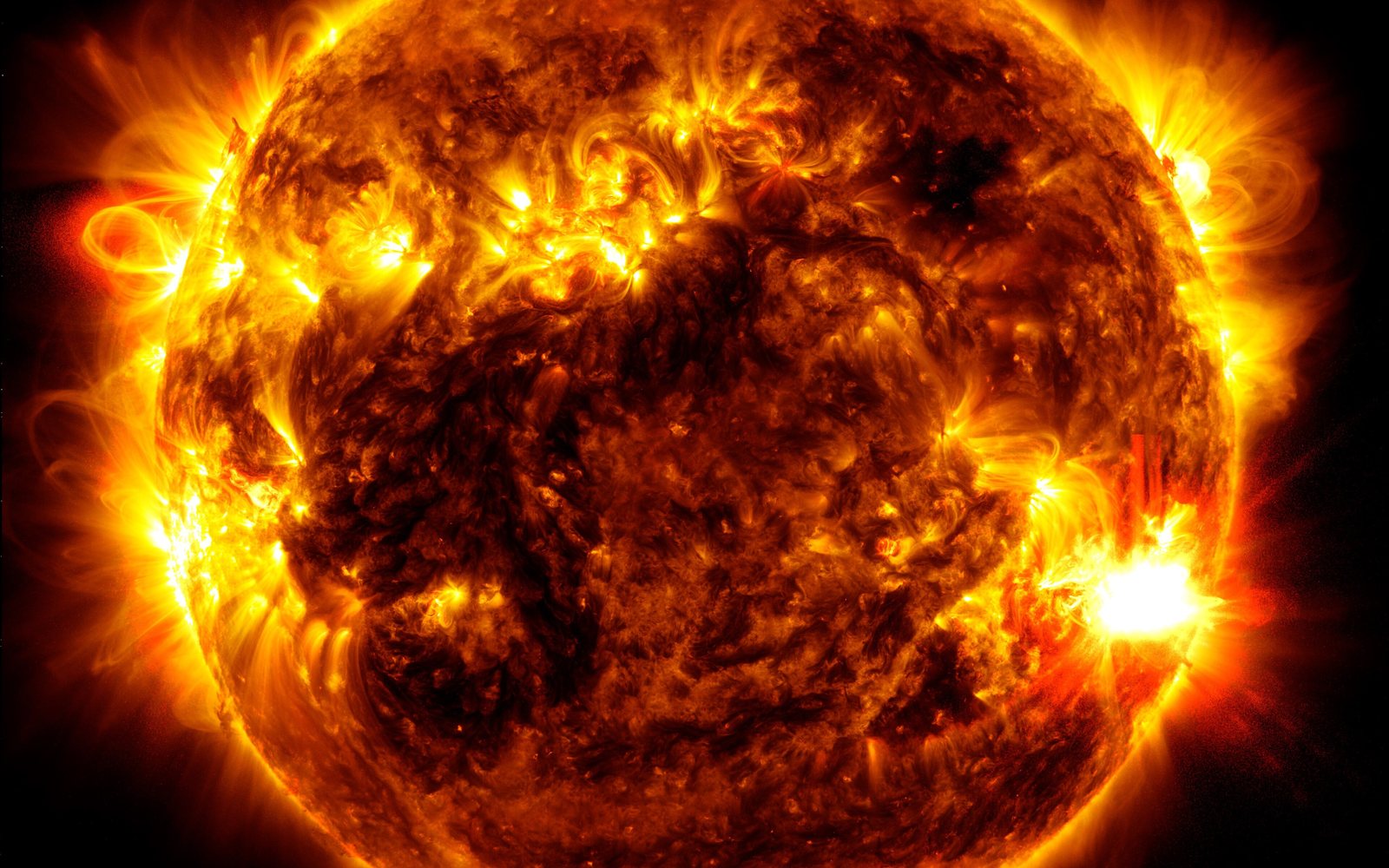
Solar flare, NASA SDO, cover for AI forecasting of solar activity (F10.7)
Solar flare, NASA SDO. Photo by NASA Scientific Visualization Studio, Public domain
All workSpace weather, sun

Forecasting the Sun's radio pulse withfinancial engineering and deep learning

F10.7 solar radio flux forecasting with log-differenced targets, PCA-compressed technical indicators, physics-based Fourier residuals, split conformal uncertainty and four-layer explainability

Treating the Sun like a stock chart: trader's tools plus deep learning beat NOAA's official 7-day F10.7 outlook by 8% across 2024.

Role
Independent researcher
When
2024 to present
Grades
G10 to G12
Recognition
  • Korea Science and Engineering Fair (KSEF), Silver
  • International Greenwich Olympiad (IGO) 2026
Best RMSE
9.704 sfuBest RMSEBest of 315 trained models, versus 15.77 sfu for the baseline LSTM (−38.5%).
Better than NOAA at 7 days, 2024
8%Better than NOAA at 7 days, 2024Model h=7 RMSE 35.48 sfu vs NOAA lead-7 RMSE 38.70 sfu across 2024.
Better than NOAA during the Gannon G5 storm
20%Better than NOAA during the Gannon G5 storm29-day window (2024-04-26 to 05-24): model h=7 32.96 sfu vs NOAA lead-7 41.40 sfu.
RMSE vs NOAA on the 5-year archive
−24%RMSE vs NOAA on the 5-year archiveOperational validation over 6,961 paired forecasts (2020–2024).
90% interval coverage with split conformal
75.9%90% interval coverage with split conformalUp from 32.3% (MC Dropout) and 44.5% (Deep Ensemble); +43.6 pp, 14.1 pp short of nominal.
Models trained
315Models trained21 variants × 3 seeds × 5 walk-forward splits, about 100 GPU hours.
Forecasts paired with NOAA
6,961Forecasts paired with NOAAExtracted from 260 archived NOAA SWPC PDF outlooks, 2020–2024.
R² with NRLMSIS
0.987R² with NRLMSISPhysical validation against the NRLMSIS atmosphere model.

In brief

The problem
F10.7, the Sun's 10.7 cm radio flux, is the simplest measurement of solar activity and one of the hardest to forecast. Errors propagate into four real-world pathways: thermospheric drag on satellites, geomagnetic storms that induce currents in power grids, ionospheric disturbances that degrade GNSS and aviation signals, and energetic-particle damage to satellite electronics. During the May 2024 Gannon G5 storm, NOAA's official outlook under-forecast the peak day by 58 sfu, with a pre-peak RMSE of 66.3 sfu.
The spark
Financial engineers spend their careers forecasting the future of a noisy series from its own past. Wonjun asked whether the same toolkit, log-returns and technical indicators such as moving averages, Bollinger Bands, RSI and MACD, could be transferred to the Sun and combined with AI to sharpen F10.7 forecasts. The project grew out of earlier climate-data work (comparing ERA5 reanalysis with Korean station observations), which first got him thinking about how much a model can be trusted against reality.
The outcome
Out of 315 trained models, the best reached an RMSE of 9.704 sfu, a 38.5% improvement over the 15.77 sfu baseline LSTM. Across 2024, the 1-day model cut error to 15.28 sfu against NOAA's 38.70 sfu 7-day lead; at the fair 7-day horizon the model's 35.48 sfu still beat NOAA by 8%. In the 29-day Gannon storm window the margin widened to 20% at 7 days (32.96 vs 41.40 sfu). Split conformal calibration raised 90% interval coverage from 32.3% to 75.9%, and the forecasts preserved the Sun's four physical periods.

Method

How it was done, step by step.

  1. 1Build a leak-free data foundation20 years of daily F10.7 (2005–2024, about 7,300 observations from Penticton, Canada), plus Carrington-phase sine/cosine encodings, split into 5 walk-forward folds with test years 2020 to 2024.
  2. 2Borrow from financeCompute 12 financial technical indicators (SMA5, SMA20, SMA60, EMA20, four Bollinger Band features, RSI14, MACD, MACD signal, MACD histogram) and compress them with PCA to the components explaining at least 95% of variance (5 to 7 orthogonal features), fit on training data only.
  3. 3Predict the change, not the levelReplace the raw sfu target with a log-difference target, rₜ = log(yₜ₊ₕ) − log(yₜ), the finance-standard log-return, which removes drift and stabilises variance across quiet and active Sun.
  4. 4Inject solar physics as a priorSubtract four physically known periods (11-year Schwabe cycle, 27.275-day Carrington rotation, 13.638-day half-Carrington, 155-day Rieger period) so the neural network only learns the residual.
  5. 5Train a 21-variant ablation grid3 architectures (2-layer LSTM, GRU, Transformer) × 2 targets (level vs log-return) × 2 feature sets (baseline vs PCA) across horizons of 1, 3, 7 and 27 days, plus Fourier hybrids, persistence and ARIMA baselines: 315 training runs over 3 seeds and 5 splits, about 100 GPU hours on consumer hardware.
  6. 6Benchmark against NOAAPair forecasts with NOAA SWPC's official 27-day outlook from 260 archived PDF reports (2020–2024, 6,961 paired forecasts) at lead days 1, 3, 7 and 26, with Diebold–Mariano (HLN) tests and a Gannon storm stress test.
  7. 7Quantify uncertainty and explain the modelCompare MC Dropout, Deep Ensembles and split conformal calibration for 90% prediction intervals, then open the model with permutation importance, Integrated Gradients, spectral (FFT) preservation and SSIM shape similarity.

01Why it matters

A single number that moves satellites and power grids

F10.7 is the solar radio flux at a 10.7 cm wavelength, measured daily in Penticton, Canada, in solar flux units. When it rises, the upper atmosphere expands and drags satellites down, geomagnetic storms push currents into transformers, the ionosphere scrambles GPS and aviation signals, and particle radiation flips bits in satellite electronics. The costs are not hypothetical: the 1989 Quebec blackout left 6 million people without power for 9 hours, the 2003 Halloween storms destroyed the ADEOS-II satellite, and in 2022 a Starlink launch lost 40 satellites to re-entry within days.

  • U.S. electricity losses estimated at $1–20 billion per extreme event scenario
  • U.S. satellite industry losses estimated at $2–80 billion per extreme event scenario
  • Source: Abt Associates (2017) report for NOAA

02The gap

Even the official forecast misses when it matters most

In May 2024 the Gannon G5 storm, the strongest in two decades, hit Earth. NOAA's official outlook under-forecast the peak day by 58 sfu, and over the pre-peak week (May 3–10) its RMSE was 66.3 sfu. Wonjun framed a question: can financial-engineering methods, built to forecast markets from their own history, be combined with AI to do better? He then made it testable on three independent axes: statistical significance against an ablated baseline, operational superiority over NOAA's real archived forecasts, and preservation of the Sun's physical spectral signature.

03Borrowing from Wall Street

Treating solar flux like a price chart

Traders compute moving averages, Bollinger Bands, RSI and MACD from price history to anticipate momentum and reversals. Wonjun computed the same 12 indicators on F10.7. Because many of them overlap (SMA20 and EMA20 correlate at 0.97, and the Bollinger midline duplicates a moving average), he compressed them with PCA into 5 to 7 orthogonal components explaining at least 95% of the variance. He also switched the target to a log-return: instead of predicting tomorrow's flux, the model predicts its rate of change, which is zero-centred and stable whether the Sun is quiet or stormy.

  • Log-difference alone cut baseline LSTM RMSE from 15.77 to 10.56 sfu
  • PCA fit on training data only, so nothing leaks from the future

04Physics as a prior

Letting eighty years of solar physics do some of the work

Earlier studies decomposed F10.7 with data-driven methods such as EMD and VMD, whose modes have no physical meaning. Wonjun instead subtracted four periods that solar physicists already know: the 11-year Schwabe cycle, the 27.275-day Carrington rotation, its 13.638-day half, and the 155-day Rieger period. The neural network then only has to learn the residual, focusing its capacity on the genuinely unpredictable part of the signal.

  • Schwabe cycle: 11 years
  • Carrington rotation: 27.275 days
  • Half-Carrington: 13.638 days
  • Rieger period: 155 days

05The experiment

315 models, one winner

To prove each ingredient mattered, he built a 21-variant ablation grid: LSTM, GRU and Transformer architectures, raw-level vs log-return targets, baseline vs PCA features, across horizons of 1, 3, 7 and 27 days, plus Fourier hybrids, a persistence model and ARIMA. Each variant was trained with three random seeds over five walk-forward splits, 315 runs and about 100 hours of consumer GPU time, with fixed hyperparameters and no tuning loop. The best model reached an RMSE of 9.704 sfu, 38.5% better than the plain LSTM baseline.

06Head to head

Beating NOAA on its own archive

Academic papers usually compare against other neural networks. Wonjun went further and digitised 260 of NOAA SWPC's archived 27-day outlook reports, producing 6,961 forecast pairs from 2020 to 2024. Across 2024, at the fair 7-day horizon, his model's RMSE of 35.48 sfu beat NOAA's 38.70 sfu by 8%; his 1-day model reached 15.28 sfu. Inside the 29-day Gannon storm window, the 7-day model beat NOAA by 20% (32.96 vs 41.40 sfu), and the 1-day model cut error by 74% to 10.89 sfu.

  • Diebold–Mariano (HLN) tests, combined with Stouffer's Z, p ≤ 0.002
  • −24% RMSE versus NOAA across the 5-year archive

07Honest uncertainty

How sure is the forecast?

A forecast without an error bar is hard to act on. Wonjun compared three ways of building 90% prediction intervals. MC Dropout (one seed, 50 stochastic passes) covered only 32.3% of real outcomes; a three-seed Deep Ensemble reached 44.5%. Adding split conformal calibration, which widens intervals using the 90th-percentile residual on validation data, lifted coverage to 75.9%. That is a 43.6-point gain, yet still 14.1 points short of the nominal 90%, a shortfall he reports openly rather than hides.

08Opening the black box

Accurate for the right reasons

Four explainability lenses checked whether the model was meaningfully accurate, not just numerically close. Permutation importance showed the most recent five days of F10.7 dominate, with financial indicators and Carrington phase contributing, and the ranking was identical across all three seeds. Integrated Gradients revealed the model shifts attention with horizon and with quiet vs storm conditions. A spectral check confirmed the four solar periods survive in the predictions with no spurious frequencies, and SSIM showed storm rise, peak and decay shapes are preserved.

09What's next

Limits, and the road to a full forecasting system

Accuracy plateaus around 45 days, a limit that helioseismic far-side imaging and CME or flare event flags may lower but chaos ultimately bounds. MC Dropout coverage drops at solar minimum, so regime-aware conformal calibration will need the next minimum (around 2031) to validate. Transfer to sunspot number reached R² = 0.78 without native training, and a full-cycle reanalysis from 1976 would need roughly ten times the GPU hours. Downstream, F10.7 forecasts tracked yearly total solar irradiance at R² = 0.85, linking the work to climate-model solar forcing.
Try it

An interactive model of the work.

The data

Results, rebuilt from the original slides.

Improvement cascadeEach ingredient lowers RMSE. Baseline is a plain LSTM with no PCA, no log-difference and no Fourier residual; the best model is the top of the 21-variant leaderboard.RMSE (sfu)
  • Baseline LSTM15.77
  • Baseline + log-difference target10.56
  • Best model9.704
2024 full year: model vs NOAARMSE across 2024. At the fair 7-day horizon the model beats NOAA's 7-day lead by 8%; the 1-day model is 60% lower than NOAA's 7-day lead.RMSE (sfu)
  • NOAA SWPC (lead 7)38.7
  • This model (h = 7)35.48
  • This model (h = 1)15.28
Gannon G5 storm window: model vs NOAARMSE over the 29-day window, 2024-04-26 to 2024-05-24. The model beats NOAA by 20% at 7 days and 74% at 1 day.RMSE (sfu)
  • NOAA SWPC (lead 7)41.4
  • This model (h = 7)32.96
  • This model (h = 1)10.89
90% prediction-interval coverageShare of actual outcomes falling inside the 90% interval, over five test years. Split conformal calibration adds 43.6 pp but remains 14.1 pp below nominal.Coverage (%)
  • MC Dropout (1 seed × 50 passes)32.3
  • Deep Ensemble (3 seeds × 30 passes)44.5
  • + Split conformal (val q90)75.9
  • Nominal target90
Walk-forward splitsEach split starts its training window one year later and is tested on a year it has never seen (training runs up to the validation year).
SplitTraining startsValidationTest
S1200520192020
S2200620202021
S3200720212022
S4200820222023
S5200920232024
How this study differs from prior F10.7 workSix dimensions on which the project departs from earlier research.
DimensionPrior F10.7 workThis study
Cross-domain featuresF10.7 history only or other solar proxies+12 financial indicators compressed by PCA
Target transformationRaw level (sfu)Log-difference (finance standard, rare in F10.7)
DecompositionData-driven (EMD, VMD, FIF) with no physical meaningPhysics-based (Schwabe, Carrington, half-Carrington, Rieger)
Uncertainty calibrationNo identified F10.7 split conformal studiesPotentially first split conformal application
ExplainabilityRMSE onlyFour-layer suite: permutation importance, Integrated Gradients, spectral, SSIM
External benchmarkNeural-network baselinesNOAA SWPC outlook (260 reports, 6,961 pairs)
Research procedureEight stages from raw data to explainable, calibrated forecasts.
  1. 1Data foundation
  2. 2Feature engineering
  3. 321-variant training grid
  4. 4Internal leaderboard
  5. 5External validation vs NOAA
  6. 6Gannon storm stress test
  7. 7Uncertainty calibration
  8. 8Explainable AI
Physical and downstream validationHow well forecasts connect to other physical quantities.
LinkR²Meaning
NRLMSIS atmosphere model0.987Physical consistency
Yearly total solar irradiance (TSI)0.85Climate-model solar-forcing proxy
Sunspot number (transfer, not native)0.78Generality to another proxy
Geomagnetic storm days0.432–3 day lead to Dst for grid resilience

Plain English

Terms worth knowing.

F10.7
The strength of the Sun's radio emission at a 10.7 cm wavelength, a daily proxy for overall solar activity.
sfu (solar flux unit)
The unit F10.7 is measured in; 1 sfu = 10⁻²² W/m²/Hz.
Log-difference (log-return)
Predicting how much a value changes in percentage terms rather than the value itself; standard in finance.
Technical indicators
Formulas traders apply to price history, such as moving averages, Bollinger Bands, RSI and MACD.
PCA
A way to squeeze many overlapping features into a few independent ones that keep most of the information.
Carrington rotation
The Sun's roughly 27-day rotation as seen from Earth, which makes active regions recur.
Walk-forward validation
Training only on the past and testing on the following year, so the model never peeks at the future.
Split conformal prediction
A calibration step that widens forecast error bars using real errors on held-out data, so stated confidence matches reality.
Integrated Gradients
An explainability method that attributes each forecast to the input features that drove it.
NOAA SWPC
The U.S. Space Weather Prediction Center, which issues the official F10.7 outlook.

Reflection

The most valuable lesson was that cross-domain ideas need rigorous proof to earn their place. Borrowing financial indicators sounded clever, but only a full ablation grid, real NOAA forecasts and explainability checks could show they help for the right reasons. Reporting the 14.1-point coverage shortfall and the 45-day accuracy plateau honestly mattered as much as the headline wins: a forecaster people can trust needs quantified uncertainty, not just a low error.
SourcesWonjun Lee, 'F10.7 Solar Radio Flux Forecasting Using Multi-Architecture Deep Learning with Financial Engineering and Multi-Period Fourier Residual under Conformal Uncertainty and Four-Layer Explainability', presentation (Cheongshim International Academy); Abt Associates (2017), Social and Economic Impacts of Space Weather in the U.S., NOAA NWS Final Report; Warren, Emmert & Crump (2017), Linear forecasting of the F10.7 proxy, Space Weather 15; Han et al. (2021), A deep learning approach to solar radio flux forecasting, Adv. Space Res. 68(7); Stevenson et al. (2022), F10.7 forecasting with deep CNN-LSTM, Processes 10(2); Jiang et al. (2024), LSTM-based F10.7 forecasting up to 45 days, Astron. Comput. 46; Zhao et al. (2026), VMD-SOBI-DLinear hybrid for medium-term F10.7 forecasting, Sol. Phys. 301; Daniell & Mehta (2023), Probabilistic solar proxy forecasting with neural network ensembles, Space Weather 21(9); Zhou et al. (2021), Informer, Proc. AAAI 35(12); Henney et al. (2012), Forecasting F10.7 with solar magnetic flux transport modeling, Space Weather 10